3 Search Algorithms
A common application of walks is in search problems. In search problems, we generally have a black box function
\[ f(x) = \begin{cases} 0 & x \in G\\ 1 & x \in G^C \end{cases} \]
where \(G \cup G^C = S\) which is the search space. We are interested in developing an algorithm to output some \(x \in G\) by querying \(f\).
Naively, one can run a stochastic process over the domain \(G\cup G^C\) and observe the system until we see an element in \(G\). The average time to succeed in this protocol is called the hitting time of \(G\), and denoted as \(HT(P, G)\). Naturally, we not only want high success rates, but we also want low mean hit times.
In the particular case of Markov chains, hitting times are a kind of stopping time (Appendix A), and are well studied in their own regard.
Formalism
Define the following
- Denote the readout at the \(n^{\text{th}}\) measurement (at \(t=n\tau\)) as \(X_n\).
- Select a target node \(\delta\)
- Probability of first hit in \(n\) steps \(F_n = P(X_n = \delta | X_i \ne \delta \forall i \in [0, n-1])\)
- Mean hit time \(\langle t_S \rangle = \sum_{i=0}^\infty i F_i\)
- Success probability in \(n\) steps \(S_n = \sum_{i=1}^{n}F_i = P(\exists i \in [0, n]| X_i = \delta)\)
- Survival probability \(=\) Failure probability \(= \mathcal{S}_n = 1 - S_n\)
- Asymptotic versions of these terms are given by taking \(n\to \infty\)
Readout in Walks
To identify whether a walker has hit the target node, we need to track the location of the walker as it evolves in time.
For the classical case, this poses no problem, as measurement does not disturb the system. In the quantum case however, we need to be a bit more careful.
A constantly measured walker will freeze the dynamics of a quantum walker. This is known as the Quantum Zeno effect. The solution for this is to measure after every \(\tau\) steps.
Semi-quantum walk
This results in what is technically a semi-quantum walk1, since measurement leads to a complete loss of coherence in the system. However, the walk between two measurement events is quantum in nature, and increasing \(\tau\) leads to the quantum features of the walk dominating. We shall however keep this at the back of our minds and refer to this walk as the quantum walk, until we reach Chapter 6.
Reduction to classical random walk with \(\tau=1\)
The quantum \(\tau = 1\) case reduces the discrete time quantum walk to a classical random walk with \(\tau=1\). Effectively, we apply a dephasing operator on the density matrix, dropping all off diagonal terms. Thus, we lose all effects of superposition, causing the classical random walk.
Plotting the readout trajectories of walkers with different parameters in Figure 3.1, we see the very clear difference in the spread between the classical readout and the quantum readout for same \(\tau\): The quantum walker spreads much faster than the classical walker, and thus scans a larger area. Similarly, note the spread between the quantum readouts for different \(\tau\)s: A larger \(\tau\) value leads to the walk behaving more quantum-like, corresponding to a larger spread for the same number of measurements.
Markov Chains and Walks
In the classical case, it is clear that the 1D SSRW is a Markov process. In Appendix B, we show that the quantum walk with measurement is also a Markov process. Consequently, we can use certain results from the theory of Markov processes to compare the two walks.
Irreducibilty and Recurrence
Under the usual definition of irreducibility (Appendix A), it is trivial that in the 1D chain, \(n = m = |i-j|\tau\) satisfies the condition. It is a well known fact that the 1D SSRW is recurrent. It is just as well known a fact that the 3D SSRW is transient2.
In the quantum case, it is not as clear whether any of the available definitions of the quantum Markov process is more or less good than the others. Thus, the transience of quantum walks depends on the exact definition we are working under3. In our definition however, it can be shown using symbolic computation4 that the walk is indeed transient. This poses an interesting problem which we shall discuss below.
Survival probability
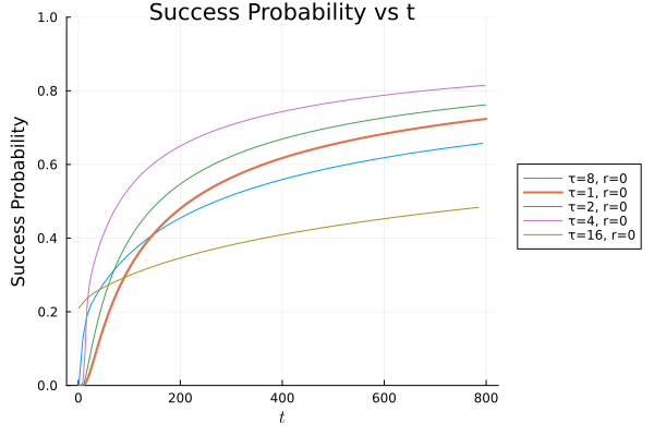
We can thus measure and plot the \(S_n - n\) curve for the quantum and classical walks to compare the efficiency of these walks in the first hit problem.
In previous work5, the analytical solution of the success rate as a function of time is found. An analytical result for discrete time walks is harder due to the nature of the walk. However, we reproduce the results for the discrete time case computationally. Figure 3.2 (a)5 shows the success rate for the continuous time quantum and classical walks, and Figure 3.2 (b) shows our results for the discrete time case.

Observations - The Tortoise and the Hare
In the continuous time case:
- The quantum walk has a fast rise in the initial phase but saturates at ~0.1
- The classical walk has a slow rise, but eventually reaches 1
In the discrete time case, solved computationally:
- Both walks do eventually reach 1
- The quantum walk shows a saturation for a while before suddenly rising again
- The classical walk shows a slow rise in the beginning phases, in contrast to the sharper rise of the quantum walk.
There seems to be an apparent difference between the discrete and the continuous time walks, where in the discrete walk, the asymptotic success reaches 1 even in the quantum case, but this is only an artifact of the finite size of the walk space. It is well known that any irreducible finite chain is recurrent6. This claim can be verified by simply increasing the size of the state space, and noting that the saturation phase in the quantum walk lasts longer.
The observations in the continuous time case can be explained by the recurrence of the walk. While the quantum walker is faster (See Chapter 2), the transient nature (See Section 3.2.1) of the walk leads to a non-zero asymptomatic failure rate. Clearly this is a problem. What this means practically, is that for the first hit problem, if the quantum walk hits the target node, it does so faster than the classical walk, but a majority of the times, it doesn’t hit the target node at all. This is reminiscent of the age-old fable of a race between the Tortoise and the Hare. The Tortoise-like classical walk is slow, but trudges on to the finish line, whereas the Hare-like quantum walk speeds away in the beginning, but falls behind.
But we want a walk that is both fast, and with an asymptotic success rate of 1. Can we give something to our Hare so that it doesn’t fall asleep?