function €(n, r₀)
    ks = map(1:n) do i
        (1/√n * [1 0; 0 0] ⊗ (S(n)*H(n))) +
        [0 0; 0 1] ⊗ I(2) ⊗ real(ket(r₀,n)*bra(i,n))
    end
    return KrausOperators(sparse.(ks))
end;5 Quantum Resetting by Superposition
From the previous discussion, it seems fruitful to consider a quantum reset of quantum walks. Just as we harnessed the power of quantum superposition to speed up the walk, can we similarly have a superposition between the reset and evolution to increase the efficiency of hitting a node? The concept is similar to that of the quantisation of the classical walk: let the resetting occur on probability amplitudes rather than probabilities, allowing for interference in areas we do not want the walker to be on. In this case however, the superposition is on the level of operations, not the walker position directly.
Our first protocol is motivated by the quantum resetting of quantum systems introduced in Anubhav Srivastava’s1 master thesis, where a similar formalism was applied to a qubit system. The faster convergence of the quantum reset system acts as the primary indicator that such a speed-up may also be visible in quantum walks.
Formalism
On a finite 1D chain of length \(2N + 1\), define the following -
- Reset operation - \(\mathcal{R}\) by the Kraus operators \(\{\mathcal{R_i} = |r_0\rangle\langle i|\}_{i\in [-N, N]}\) on \(\mathcal{H}_W\)
- Evolve operation - \(\mathcal{U}\) by the unitary operation \(S\circ H\) on \(\mathcal{H}_C\otimes\mathcal{H}_W\)
- Attach another two level coin - states denoted by \(|0\rangle\) and \(|1\rangle\). Resulting state lies in \(\mathcal{H}_R\otimes\mathcal{H}_C\otimes\mathcal{H}_W\)
- Controlled reset operation - \(\mathcal{E}\) by the Kraus operators \(\{\mathcal{E}_i = |0\rangle\langle 0|\otimes I_2 \otimes \mathcal{R}_i + \frac{1}{\sqrt N} |1\rangle\langle 1|\otimes \mathcal{U}\}_{i\in [-N, N]}\). See Appendix C for proof that this set of Kraus operators represents a CPTP map.
- A reset coin operator \(\Gamma(\gamma) = \begin{bmatrix}\sqrt{1-\gamma} & \sqrt{\gamma} \\ \sqrt{\gamma} & -\sqrt{1- \gamma}\end{bmatrix}\) on \(\mathcal{H}_R\)
Quantum Reset
One step of the resulting walk is defined as
\[\mathcal{E} \circ \left(\Gamma \otimes I_2 \otimes I_{2N+1}\right)\]
Once again, the hitting protocol is found by measuring the walker position after \(\tau\) time steps.
Although the protocol is similar to the motivation, the current problem we are considering of the first hit time has drastically changed the methods of exploration and the property we want to optimize. Where previously we only probed the convergence time, here we also want to maximize the probability of hitting the target node.
Interpretation of \(\gamma\) and dependence on initial condition of the coin
In the stochastic resetting \(\gamma\) is understood as the “rate” of resetting. However, this is no longer accurate for the quantum case. Consider the case for \(\gamma = 0\). Then, the Gammamard operator \(\Gamma = \begin{bmatrix}1 & 0\\ 0 & -1\end{bmatrix}\). This does not automatically imply that the reset never occurs; we also require that the initial state of the reset coin is \(|0\rangle\). If the initial state of the reset coin is \(|1\rangle\), this corresponds to the always reset case. Thus, \(\gamma\) is better understood as the probability that given the last step was a Reset, what is the probability this step is an Evolve, and vice versa. Thus, it is not immediately obvious how we can compare the reset mechanisms for a given \(\gamma\). Nor is it obvious how the initial state of the reset coin finally affects the success probability and such, and needs to be numerically checked.
Resetting of the walker coin
In our specific formalism (Section 5.1), we have only applied the reset operation on the walker \(\mathcal{H}_W\). One could also reset the walker coin \(\mathcal{H}_C\) and see what happens. In our current formalism, there is no entanglement broken between the two coins, but there is no a priori understanding of how this may (or may not) affect the walk.
Computational Implementation
Implementations of \(\mathcal{U}, U, H\) follow as before. The \(\mathcal{E}\) operation is implemented as
The Gammamard operation \(\Gamma\) is defined as
Γ(γ) = [
    √(1-γ)  √γ;
    √γ      -√(1-γ)];
We take the initial reset coin to be \((S(-\pi/2)\circ\Gamma(\gamma))|0\rangle\) for the same reason as in the quantum walk
reset_init(γ) = [1 0; 0 -1im]*gammamard(γ)*ket(1, 2);Results
What the walk looks like
For the specific choice of initial reset coin as \(1/\sqrt{2}\left(|0\rangle - i|1\rangle\right)\) and \(\gamma=0.2\), the quantum reset walk looks like Figure 5.1.
Results and Discussion
As discussed in Section 5.1.1, we need to vary the three parameters, \((\alpha, \phi, \gamma)\), and see what happens. Thus, we plot the success curves for a few sets of parameters (Figure 5.2), and find the minimum mean time of hit for each fixed parameter (Figure 5.3).
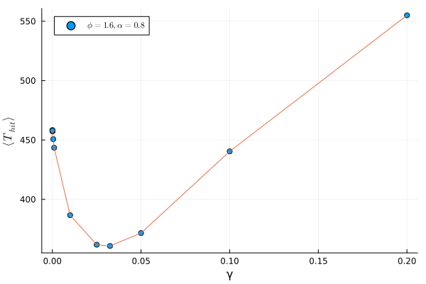
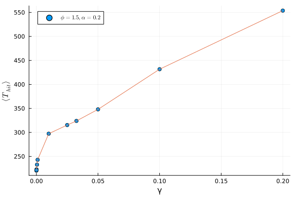
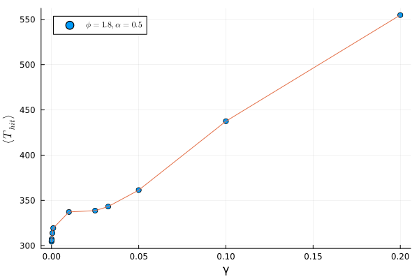
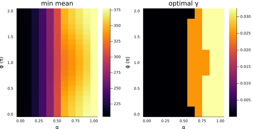
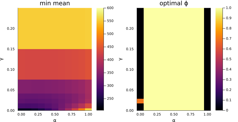
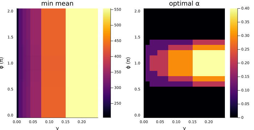
As we can see, the mean time of hit even for the best set of parameters (within the ranges explored) is not better than the optimal time for the stochastic reset protocol. This result however may not hold true for other values of \(\tau\), and more work is necessary to conclusively state that there isn’t (or is) any speedup achieved here.
Optimal Parameter Values
| \(\alpha\) | \(\phi\) | \(\gamma\) |
|---|---|---|
| \(0.0\) | \(0.0\) | \(10^{-5}\) |
The Issue of Non-Unitarity
One drawback of this formalism is its complexity. Whereas the stochastic reset proceeded by a unitary evolution between measurement events, the quantum reset protocol is inherently a non-unitary operation. This makes analysis more complicated.
The difficulty doesn’t only lie in analytical complexity, but also in simulations, where simulating the quantum reset quantum walk takes much longer. This can be attributed to the larger system size (size of \(\rho = 16N^2\)), and due to the increased number of matrix multiplications and additions (\(2N\) matrix multiplications of size \(4N\times 4N\) (\(64N^3\) multiplications and \(64N^3 - 16N^2\) additions) followed by \(N\) matrix additions ($16N^2 additions) which finally consists of \(128N^4\) multiplications and \(128N^4\) additions for one step of the quantum reset walk, as compared to \(2\cdot 8N^3\) multiplications and \(2 \cdot 8N^3 - 4N^2\) additions. Even ignoring the additions, the quantum reset walk is \(\mathcal{O}(N^4)\) whereas the stochastic reset walk is \(\mathcal{O}(N^3)\) to simulate. For any reasonably large cycle (to avoid finite size effects), this cost makes simulating the walk for different parameters extremely tedious.
Therefore, although we have been able to introduce a superposition between the two operations, and we have decoupled the resetting from the measurement, we require a unitary protocol to efficiently perform the walk.