init_coin = 1/√2 * (ket(1,2) - 1im * ket(2,2));2 Quantum Walks
Introduction
Quantum walks are defined analogous to the classical walks. First, our walker is quantum mechanical, and the position of the walker can be a superposition of the nodes. Thus, we define the state of the walker to be a superposition of the node states \(|i\rangle\).
\[|\psi\rangle = \sum_i c_i|i\rangle\]
Let this Hilbert space be denoted as \(\mathcal{H}_W\). The projection of the state on some node \(i\) given by \(|\langle i | \psi\rangle|^2 = |c_i|^2\) is understood as the probability that the walker will collapse to the state \(|i\rangle\) on measurement.
To define the evolution of the node, we look back at the transition matrix \(P_{ij}\). Thus, we would define an operation in the following manner -
\[O |i\rangle = \sum_j \sqrt{p_{ij}} |j\rangle\]
The walk proceeds by repeated application of \(O\).
While this expression is enough to define the walk, it is not immediately clear how one would explicitly realize such an operation. Multiple formalisms define such walks, but we shall use the coined quantum walk formalism which is very natural for regular graphs, as is the case for the 1D chain. Note that for the symmetric walks on nD lattices, like the 1D chain, the tight-binding model is already a well understood continuous time quantum walk. However, we prefer a discrete time formalism.
Coined Quantum Walk for 1D Chain
For the 1D chain, given a specific node, there are only 2 other nodes connected to it. Thus, we can add a 2 level system, which “decides” which node the walker jumps to. More formally, we attach a 2 level qubit system to the walker whose bases are denoted by \(|0\rangle\) and \(|1\rangle\). Let us denote this Hilbert space as \(\mathcal{H}_C\)
Thus, we can define the shift operation as
\[S |0\rangle|i\rangle = |0\rangle|i-1\rangle; S |1\rangle|i\rangle = |1\rangle|i+1\rangle\]
How would we define such an operation explicitly?
Controlled shift operation
\[S = |0\rangle\langle 0|\otimes S_L + |1\rangle\langle 1|\otimes S_R\]
Where \(S_L\) and \(S_R\) are defined as
\[S_L |i\rangle = |i-1\rangle,\ S_R |i\rangle = |i+1\rangle\]
Note that \(S\) operates on \(\mathcal{H}_C\otimes\mathcal{H}_W\), whereas \(S_L\) and \(S_R\) operate on \(\mathcal{H}_W\) only.
The superposition in the two choices at each step is recovered by putting the coin into a superposition of its basis states. This is achieved via a coin operator, which is commonly defined as \(H\otimes I\), where \(H\) is the single qubit Hadamard operator.
Quantum Walk
Thus, one step of the quantum walk is defined as \(S \circ H \otimes I\), operating on a two level coin and an \(n\) level system, with the state of the whole system lying in \(\mathcal{H}_C\otimes\mathcal{H}_W\)
Let us explicitly write down two steps of the walk
\[H\otimes I (|0\rangle |0\rangle) = \frac{|0\rangle |0\rangle + |1\rangle |0\rangle}{\sqrt 2}\] \[S\left(\frac{|0\rangle |0\rangle + |1\rangle |0\rangle}{\sqrt 2}\right) = \frac{|0\rangle |-1\rangle + |1\rangle |1\rangle}{\sqrt 2}\] \[H\otimes I \frac{|0\rangle |-1\rangle + |1\rangle |1\rangle}{\sqrt 2} = \frac{|0\rangle |-1\rangle + |1\rangle |-1\rangle + |0\rangle |1\rangle - |1\rangle |1\rangle}{2}\] \[S \frac{|0\rangle |-1\rangle + |1\rangle |-1\rangle + |0\rangle |1\rangle - |1\rangle |1\rangle}{2} = \frac{|0\rangle |-2\rangle + (|1\rangle + |0\rangle) |0\rangle - |1\rangle |2\rangle}{2}\]
Repeated application of Coin Operator
Note specifically the repeated application of the coin operator. If the coin operator is not applied in step 3, our state will end up in \(\frac{1}{\sqrt{2}} (|0\rangle|-2\rangle + |1\rangle|2\rangle)\) which is not what we wanted. This is because the application of the controlled shift operation entangles the coin and the walker systems, and thus there is no superposition in each term of the system
Computational Implementation
We show 2 ways to implement the Quantum walks, which are both interesting in their own ways. But the foremost thing to tackle would be how to store an infinite vector and an infinite dimensional operator. Since we cannot do either of these simply, we instead limit our walk to a node space of \(2n\), and use periodic boundary conditions.
Other Boundary Conditions
One could pick other boundary conditions too, such as the open or the absorbing boundary conditions, but both of these BCs lead to non-unitary operations, which complicate the definition and application of the gate.
Matrix formalism
The first and more immediate method is to simply write down the matrix equivalent of the above operations. For the visualization of the implementations, we will assume that the walk occurs in a 1 D chain of size 4.
The coin is preferred to be in the \(\frac{1}{\sqrt2}(|0\rangle + i |1\rangle)\) state when we start so that the walk proceeds symmetrically1.
The coin operator is trivial to write,
H = KrausOperators([sparse(hadamard(2)⊗I(4))]);The left and right shift operators can be defined in the following manner.
R = collect(Tridiagonal(fill(1., 3), zeros(4), zeros(3)))
R[1, end] = 1
L = collect(Tridiagonal(zeros(3), zeros(4), fill(1., 3)))
L[end, 1] = 1
Thus, the shift operator is defined as
S = KrausOperators([sparse(proj(ket(1, 2)) ⊗ L + proj(ket(2, 2)) ⊗ R)]);Thus, we can repeatedly apply \(S\circ H\) to the initial state and accumulate the results.
init_state = proj(init_coin ⊗ ket(2,4))
ψ = [[init_state]; accumulate(1:40, init=init_state) do old, _
    H(S(old))
end];
Now we can plot the readout statistics by partially tracing out the coin, and plotting the diagonal. Figure 2.1 is a walk on 61 nodes.
Quantum Walks are not random
Note, this is a single walker, not an ensemble of walkers as is the case in classical random walks. Quantum walks (without measurement), are completely deterministic.
Circuit Formalism
While the matrix definition of the Quantum Walks are easy to formalise and understand, finally these need to be simulated on some sort of device which may require us to reformulate it. Further, we try to ensure that the reformulation allows for easy additions of other dynamics which we may want to study.
The advantages of using a Quantum Computer over a classical computer for a quantum walk should be obvious. The problem however is that the quantum walk is over a high dimensional space, and we rarely have access to such high dimensional systems which we can control easily. Instead, we need to simulate such a system using the accessible 2 level systems available in quantum computers.
Let us define the basic components of our walk.
Nodes
- Each numbered node is then converted into its 2-ary \(n\) length representation denoted by \((x_i)\). \(n\) is chosen such that \(2^n\) > \(N\)
- These bitstrings are encoded into an \(n\) qubit computer, where each basis state in the computational basis corresponds to the node with the same bitstring.
- The amplitude of a particular basis corresponds to the amplitude of the walker in the corresponding node
Coin
- The Walk Coin is a two level system, as usual
Edges and Shifts
- Since shifts are only to adjacent nodes, the left (right) shift is equivalent of subtracting (adding) 1 from the bitstring of the state.
- From the Quantum adder circuit, we can set one input to be \((0)_{n-1}1\) and reduce the circuit to get the Quantum
AddOnecircuit. Shown below is the circuit for \(n=4\) \((N=16)\) - We can similarly construct the
SubOnecircuit, but that is simplified by noting that theSubOnecircuit is simply the inverse of theAddOnecircuit, and this corresponds to just inverting the circuit (all gates are unitary). - The circuits for the left (and right) shift operation is shown in Figure 2.3 (and Figure 2.2)
rightshift(n) = chain(
    n,
    map(n:-1:2) do i
        control(1:i-1, i=>X) end...,
    put(1=>X)
)
leftshift(n) = rightshift(n)';YaoPlots.plot(rightshift(4))
YaoPlots.plot(leftshift(4))
- The controlled shift operation is encoded by controlling on the coin qubit as seen in Figure 2.4.
shift(n) = chain(n+1,
    control(1, 2:n+1 => rightshift(n)),
    put(1 => X),
    control(1, 2:n+1 => leftshift(n)),
    put(1 => X),
)

YaoPlots.plot(shift(4))
Coin operator
We can add the coin operator as usual on the first rail (Figure 2.5).
coin(n, c=Yao.H) = chain(n+1, put(1 => c))
YaoPlots.plot(coin(0))
Evolve Circuit
Putting these together, we get the operation for a single step of the evolution as below. Note that the top qubit rail is that of the coin, and the rest are those of the simulation of the system.
This circuit (Figure 2.6) can be repeated to achieve any number of steps.
evolve(n) = shift(n) * coin(n)
YaoPlots.plot(evolve(4))
Prepare circuit
While we can already simulate the walk, a very useful helper function that we can define is the prepare circuit.
Quantum registers are often initialized to the 0 state, and it is also easy to restart the walk from the 0 state. However, we often like to start the walk in the center of the chain instead of at node 0. Also, the coin is preferred to be in the \(\frac{1}{\sqrt2}(|0\rangle + i |1\rangle)\) when we start so that the walk proceeds symmetrically1.
Hence, to perform these steps, we define the following prepare subroutine (Figure 2.7).
prepare(n) = chain(
    n+1,
    put(1=>Yao.H),
    put(1=>Yao.shift(-π/2)),
    put(n+1=>X)
)

YaoPlots.plot(prepare(3))
Plotting the walker distribution (Figure 2.8) as before, we see that the two implementations are equivalent.
Properties of the walk
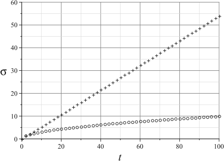
Similar to the classical random walk, the mean \(\mu(t) = 0\), if the initial state of the coin is \(\frac{1}{sqrt{2}}(|0\rangle - i|1\rangle\). If the coin is in another state, then the walk is biased towards a direction.
A more interesting feature is that the standard deviation \(\sigma(t) = 0.54 t\)1. Compare this with the classical random walk (Figure 2.9), the quantum walk has a quadratic speed up. This is the reason for the quadratic speedup commonly seen in the Grover search and other Monte Carlo problems.
Why the speed up?
We have seen that the quantum walk spreads ballistically and therefore shows a quadratic speed-up over the classical walk. This can be explained much more clearly from the continuous time versions of these walks2.
In the classical case, we have the master equation -
\[\frac{\partial P(x, t)}{\partial t} = \gamma\left[P(x+1, t) + P(x-1, t) - 2P(x,t)\right]\]
In the quantum case, we have the Schrodinger equation -
\[-i\frac{\phi(x,t)}{\partial t} = \gamma\left[\phi(x+1, t) + \phi(x-1, t) - 2\phi(x,t)\right]\]
These look almost the same, but the most important difference is that where the classical walk is an evolution of probability distributions, the quantum walk is an evolution of probability amplitudes; where probability distributions must be positive, probability amplitudes may be negative, or even complex. This is the key ingredient that allows us to introduce interference within the forward-moving and backward-moving parts of the wave, such that the walker concentrates on the edges rather than the middle, thereby exploring the space faster.