γ = 0.2
U1 = sparse(SymTridiagonal(fill(0., 31), fill(0.5, 30)))
R = fill(0., (31, 31))
R[21,:] .= 1
U = sparse((1-γ) * U1 + γ * R);4 Stochastic Resetting
The crux of the matter is this. The quantum walk is fast in the initial phase, but eventually saturates asymptotically to a success rate of < 1. This means that some of the walkers hit the target, and others do not. If that is the case, is it possible to restart the walk when it starts saturating? That is, can we restart the walk for the walkers that have not yet hit the target after \(r\tau\) time?
For such dynamics, we will need to reformulate the walk slightly.
Formalism
A reset of the walker (classical or quantum) implies that the walker returns to its initial state, and the walk dynamics continue from there.
However, we can vary when we reset the walker by considering multiple reset processes. That is, we can vary the distribution from which we sample the times between two resets. A common reset process is the Poisson reset, where the reset times are modelled as a Poisson process with some parameter \(r\). This is particularly convenient in the case of continuous time walks1.
For the discrete walks, the geometric distribution is more natural.
\[t_{r} - t_{r-1} \sim \text{Geom}(\gamma)\]
Thus, at each step, there is a \(\gamma\) probability of reset. This results in different dynamics, which can be seen in subsequent subsections, but it has an equally drastic effect on the recurrence of the walk.
Recurrence and Resetting
In the geometric resetting case, it is clear that \(P^n_{00} \ge \gamma\), and hence \(\sum_n P^n_{00} \ge \sum_n \gamma\) which diverges as \(n \to \infty\). Thus, regardless of the initial walk, the final walk will definitely be recurrent for all irreducible walks (See Appendix A). Thus, the motivation for resetting the quantum walk which is transient should be immediately clear.
Stochastic Reset Classical Walk
In the classical case, the transition probabilities change to
\[ p_{ij} = \begin{cases} (1-\gamma) \cdot 1/2 & |i - j| = 1 \\ \gamma & j = r_0 \\ 0 & \text{otherwise} \end{cases} \]
Thus, the new transition matrix is modelled as
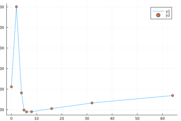
where U1 is the unchanged walk matrix and R is the reset matrix. We plot the probability distribution of the stochastic reset classical walk in Figure 4.1.
Stochastic Reset Quantum Walk
In the quantum case, the evolution changes from unitary dynamics to a non-unitary CPTP map of the following form.
\[O_{SR}(\rho) = (1-\gamma)\left(U\rho U^\dagger\right) + \gamma |r_0\rangle\langle r_0|\]
where \(U\) is the walk unitary. Plotting this walk in Figure 4.2, we see certain similarities with the stochastic reset classical walk.
function srqw(n, γ)
    R = collect(Tridiagonal(fill(1., n), zeros(n+1), zeros(n)))
    R[1, end] = 1
    L = collect(Tridiagonal(zeros(n), zeros(n+1), fill(1., n)))
    L[end, 1] = 1
    U = KrausOperators(
        [sparse(proj(ket(1, 2)) ⊗ L + proj(ket(2, 2)) ⊗ R)]
    )
    init_coin = 1/√2 * (ket(1,2) - 1im * ket(2,2))
    H = KrausOperators([sparse(hadamard(2)⊗I(n+1))])
    init_state = proj(init_coin ⊗ ket(n÷2 + 1, n+1))
    ψ = [[init_state]; accumulate(1:40, init=init_state) do old, _
        (1-γ)*H(U(old)) + γ*proj(init_coin ⊗ ket(n÷2+6, n+1))
    end]
end;Effect of Resetting on First Hit problem
For this analysis, we will consider the simpler “sharp reset” formalism2, where the reset time is sampled from a distribution
\[t_r \sim \delta(t-r\tau)\]
Therefore, we restart after \(r\) measurement events (at \(t = r\tau\)). Once we understand the effect of this kind of reset, gaining intuition for reset times sampled differently is easier.
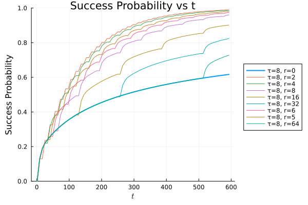
The success probability versus time can now be plotted (Figure 4.3 (a))2 for the reset case.
Now we see that the success probability is drastically increased for both cases, but due to the ballistic nature of the quantum walk, we see that the reset quantum walk performs much better than the classical walk.
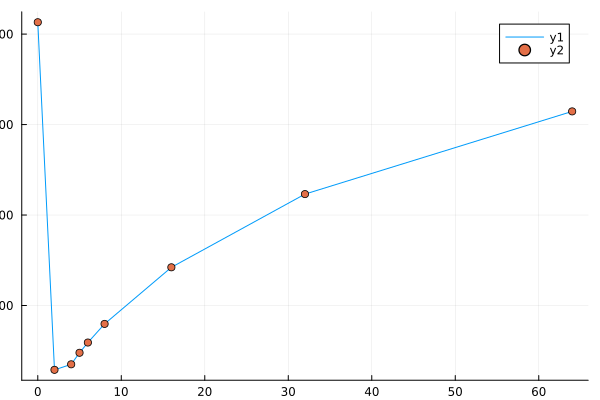
For a better understanding of the performance of the reset quantum walk with reference to changing reset rates (\(r\)) and measurement times (\(\tau\)), we can plot (Figure 4.3 (b))2 the mean first hitting time versus these parameters.


Observations
- Deterministic restart leads to zero asymptomatic failure rate
- Eager restarting leads to walker never reaching \(\delta\), reducing success rates drastically
- Cautious restart reduces the effect of restart, reducing success rates.
- There exists an optimal \(r\), but this needs to be optimized, which is nontrivial for general \(\tau\) and graph structures.
Can stochastic restarting be better than sharp reset?
No, because even if \(\langle r\rangle = r_{\text{optimal}}\), \(\langle t_f\rangle > \langle t_f\rangle_{\text{optimal}}\) due to the non-monotonic nature of the curve
Sharp Reset for Discrete time walks
For discrete time walks, the sharp reset walk is given by
\[|\psi_t\rangle = U^{t - r_l\tau} (|c_\text{init}\rangle \otimes |0\rangle)\]
where \(r_l \tau\) was the time of last reset.
Equivalently, in the circuit model, the reset circuit is considered to be a measure followed by post process where we apply the appropriate unitary rotation to rotate to \(|\psi_0\rangle\).


Our results are plotted in Figure 4.4 where the circuit formalism is run multiple times, and in Figure 4.5, we pick the diagonal term from the matrix formalism as the infinite limit. Note the similarity between the continuous and discrete curves. However, also note the difference between the non reset curve, where in the discrete case, success probability still reaches 1, this can be attributed, as before, to the finiteness of the walk space.
The Problem in the Solution
As discussed before, reset rates which are very high or low can end up being detrimental to the success times of the walk. Secondly, there is no clear path as to how to optimize the reset parameter for arbitrary graph structures.
A more fundamental problem with this protocol is the requirement of measuring at intermediate steps, and resetting accordingly. This measurement leads to a complete loss in coherence of the quantum walk. Thus, while the walk is fully quantum between measurements, measurement leads to a semi-quantum walk corresponding to a slowdown. Thus, fully quantum protocols such as the Grover search may not directly benefit from this resetting protocol. Therefore, we require a quantum resetting protocol as compared to the classical resetting mentioned here.