IDC402 Non Linear Dynamics
First Order Systems
\[\left\{\frac{dx_i}{dt} = f_i([x_j])\right\}\]In the simplest case,
$\frac{dx}{dt} = f(x)$
where $f$ has no explicit time dependance.
Consider $f(x) = sin(x)$. For this, the solution fo the diff eq is
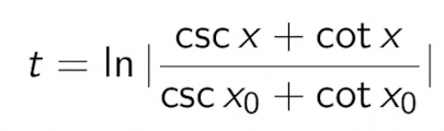
Which is a pain to evaluate, and does not give much insight.
Vector Fields
We can also represent the differential equation to be a vector field, which tells us the velocity vector on a line.
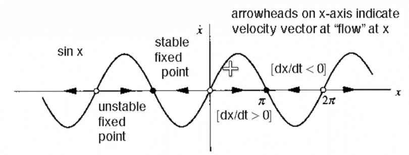
- the sign of $\dot x$ tells us which direction the flow is
- When $\dot x$ is 0, it is a fixed point $x^*$.
- Both of the above tell us which points are stable. They are those where $\dot x$ is decreasing at $x^*$
Linear stability analysis
Define
$\eta(n) = x(t) - x^*$ as a perturbation around $x^*$
Then, $\dot \eta = f(x) - 0$
But, $f(x) = f(x^* + \eta) = f(x^*) + \eta f’(x^*) + \mathcal{O}(\eta^2)$
But $f(x^*) = 0$, and $f(x) = \dot \eta$
Hence,
\[\dot \eta = \eta f'(x^\*)\]Which has a solution
$\eta = \eta_0 \exp(f’(x^*) t)$.
Stability
Hence the fixed point is
$\begin{cases}
\text{Stable} & f’(x^) < 0
\text{Unstable}&f’(x^) > 0
\text{Non linear analysis necessary}&f’(x^*)=0
\end{cases}$
Characteristic Time Scale
$\tau = \frac{1}{\vert f’(x^*)\vert}$
Population Growth
\[\frac{dN}{dt}=rN(1 - N/k)\]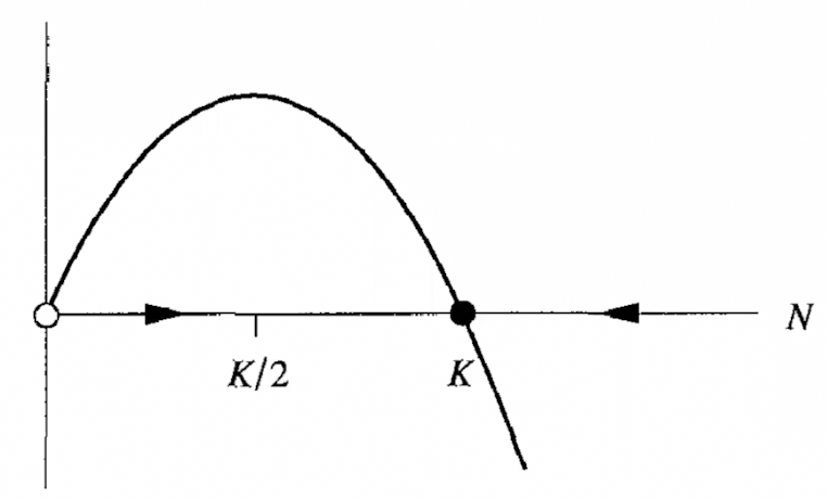
Fixed points are $N = 0$ (unstable) and $N = k$ (stable)
The flow accelerates from $0$ till $K/2$, then decelerates till $K$ and then stops.
RC Circuit
\[\dot Q = \frac{V_0}{R} - \frac{Q}{RC}\]$Q^*= V_0C$
Existance of solutions in time
Consider $\dot x = x^2 + 1$. With $x(0) = 0$, the solution is $x = tan(t)$ which exists only in $t\in(-\pi/2, \pi/2)$.
Therefore, the system blows up to infinity in finite time.
Impossibility of Oscillations
For a vector field on a line,
- Trajectories can either increase, decrease, or remain constant
- Hence, no periodic solutions to $\dot x = f(x)$
- Fixed points are either attractors or repellors
Mechanical Analogue - Over damped systems
\[m\ddot x = F(x) - b\dot x\]If $b\dot x\gg m\ddot x$,
\[\dot x = F(x)/b\]which is a flow on a single line.
$F(x)$ as a “Potential”
As in previous section, $f(x)$ can be considered as a “force” on a particle, but the particle is highly damped (think: in a highly viscous fluid).
Hence, plotting $F(x)$ tells us a “mountain” to ascend or descend.
Bifurcations
While the maps are simple, We can still get bifurcations by varying some parameter.
Bifurcations can either be points where
- Fixed points created/destroyed
- Fixed points exchange stability
See [2022-01-18#Bifurcations] for more.
Tangent Bifurcation
Consider
\[\dot x = x^2 + r\]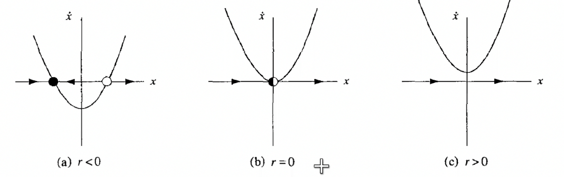
Here, we see a saddlenode bifurcation, or tangent bifurcation at $r = 0$
This is very similar to [2022-02-01#Tangent Bifurcation].
A more complicated Example
\[\dot x = r - x - e^{-x}\]The trick is to plot $r-x$ and $e^{-x}$, and to see for what value of $r$ it intersects.
Since intersection must be tangential, $\frac{d(r_c-x)}{dx} = \frac{d e^{-x}}{dx}$ at point of intersection $x^*$
Hence, $e^{x^*} = 1$ is the point of intersection. That is, $x^* = 0$.
But also, $r_c-x^* = e^{-x^*}$, which implies $r_c = 1$
Normal forms
For tangent bifurcations, $f(x, r)$ generally looks like $r \pm x^2$. This comes from the taylor expansion and that $f = 0$ and $f’ = 0$ at $(x^*, r_c)$.
Transcritical Bifurcations
Now consider a Normal form of type
\[f(x) = rx - x^2 = x(r-x)\]In this case, the $\dot x$ vs $x$ plot moves horizontally and vertically.
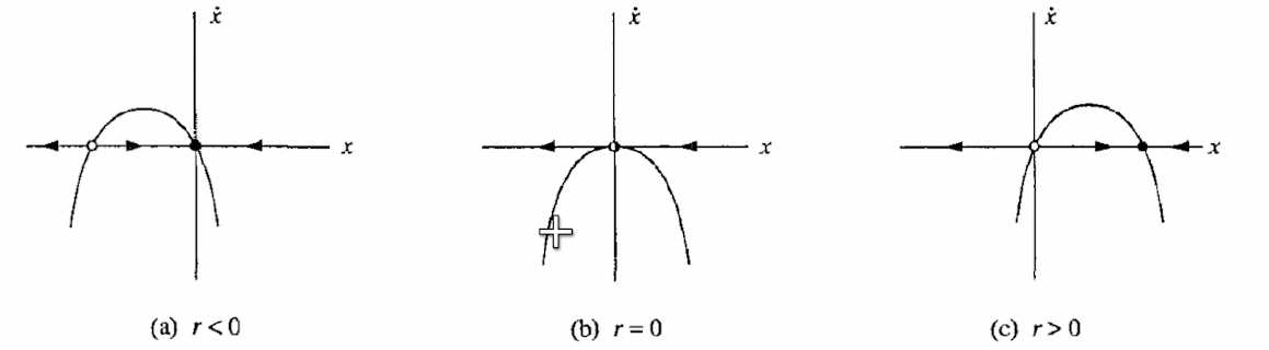
- $x^* = 0$ is always a fixed point.
- the other point is $x^* = r$
From linear stability analysis,
$f’(x, r) = r - 2x$ implies
- $x^* = 0$ is stable when $r<0$ and unstable otherwise
- $x^* = r$ is stable when $-r<0\implies r>0$ and unstable otherwise
To get to a normal mode, we can take taylor expansion of $f$ and then make a change of variable to bring it to the form $\dot x = rx-x^2$. From there, $r=0$ is the point of transcritical bifurcation, as $x^*=0$ is always a solution.
Supercritical Pitchfork bifurcations
The normal mode is of the form
\[\dot x = rx-x^3\]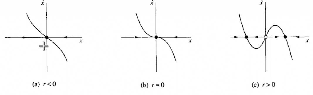
- Fixed points are $0, \pm \sqrt{r}$. Hence, only one fixed point for $r<0$
- From linear stability, $0$ is stable for $r<0$ and unstable after. $\pm\sqrt{r}$ is stable for $r>0$
Critical Slowing down
However, at $r=0$, linearity vanishes, but $x^* = 0$ is still weakly stable, in that perturbations do not decay exponentially fast, but only algebraically fast. This is known as Critical Slowing down
These are also called second order phase transitions.
Subcritical Pitchfork bifurcation
\[\dot x = rx+x^3\]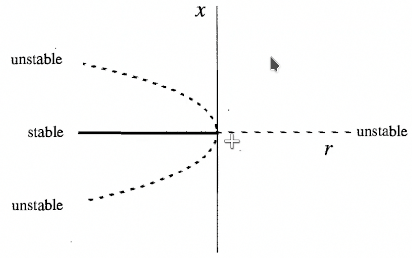
However, this is rare in physical systems and there’s not much to see in this system. Hence, we add a -ve term
\[\dot x = rx + x^3 -x^5\]gives a saddlenode bifurcation for $\vert x^*\vert \gg 0$