HSS646 Principles of Economics

Thursday, January 27, 2022

Budget Line

$P_1x_1 + P_2x_2 \le m$ $P_1x_1 + P_2x_2 = m$ where, $P_i$ is price of $i$ with quantity $x_i$ and $m$ is income.

Since income and $P_i$ is constant,

$P_1 dx_1 + P_2 d x_2 = 0$ Hence, $\frac{dx_1}{dx_2} = -\frac{p_2}{p_1}$

This is the slope of the budget line.

Variation in budget lines

Therefore, the budget curve changes as income or price levels change.

Income changes

This shifts the line to the right (left) as income increases(decreases).

Slope remains same

Price Changes

When price changes, the intercept moves towards(away from) origin as price increases(decreases).

$

\text{Slope}

$ changes linearly in $P_1$ and inversely $P_2$, but remains negative.

Effect of Tax, Subsidy and Rationing

What does imposition of tax mean to a customer?

Price of good increases. Hence, budget line changes, as above

Subsidy on quantity

Price of good decreases. Hence, budget line changes, as above

Rationing

Along with the above budget line equality, we have additional constraint $x_i\le x_i^*$

Indifference curve

They cannot intersect

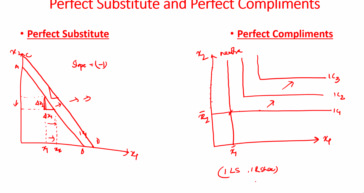
Perfect substitute and Compliments

• Substitutes - slope is 1 of budget curve
• Perfect Compliments - L shaped budget curve

Consumer Choice and Consumer Equilibrium

\(u = f(x_1, x_2) = k\) \(du = \frac{\partial{u}}{\partial{x_1}} dx_1 + \frac{\partial u}{\partial x_2} dx_2\) \(\frac{\frac{du}{dx_1}}{\frac{du}{dx_2}} = -\frac{dx_2}{dx_1}\) \(\frac{Mu_1}{Mu_2} = -\frac{dx_2}{dx_1}\)

Equal marginal Principle

Aim is to maximize utility subject to budget curve.

Hence, we define Composite utility function using the lagrange multiplier definition.

\[P(\{x_i\}) = U(\{x_i\}) - \lambda \left(\sum_i p_i x_i - M\right)\] \[\frac{\partial{F}}{x_i} = \frac{\partial{u}}{\partial x_i} - \lambda p_i = 0\]

Hence,

\[\frac{\partial u}{\partial x_i} = \lambda p_i\] \[\frac{mu_i}{p_i} = \lambda = \frac{mu_i}{p_i}\]

Hence, $\frac{Mu_1}{Mu_2} = \frac{p_1}{p_2}$

$MRS_{x_1, x_2} = \frac{Mu_1}{Mu_2}, \frac{p_1}{p_2}$

$MRS$ is the slope of the indifference curve

$\frac{p_1}{p_2}$ is the slope of budget curve.

Hence, the equilibrium point is when slope of indifference curve is equal to slope of budget line. Therefore, E is where the budget line is tangential to the indifference curve.